Calculating Fiber Loss and Distance
12/10/2018
INTRODUCTION
Fiber optics has been providing
- Fiber optics provides exceptional bandwidth and can carry many signals concurrently.
- Fiber optics is immune to electromagnetic interference.
- Fiber optics produces no electromagnetic emissions.
- Fiber optic cable does not corrode as rapidly as copper-based cabling.
- Fiber is resistant to eavesdropping.
- Fiber’s high bandwidth makes it virtually “future proof”.
- Fiber has the capability to operate in conjunction with any current or proposed LAN/WAN standard.
- Fiber is lightweight.
And, working with fiber keeps getting easier. New termination techniques, new splicing techniques, and new Small Form Factor (SFP) connector/termination products are making life a lot simpler for fiber installers. It is expected that costs for integrating fiber will be at par with Category 5 within a few years. Considering fiber’s many advantages, it is time to start planning ahead.
FIBER CABLE PHYSICAL STRUCTURE
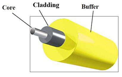
Fiber optic cable consists of three components:
- Core – A very narrow strand of
high quality glass. - Cladding – High quality glass with a slightly different index of refraction (usually within 1 - 2%) of the core’s.
- Buffer/Outer Jacket – Usually constructed from plastic and/or coverall fibers (depending on the specification and use for the fiber).
The light signal is injected into the fiber via an LED, VCSEL or laser. For installations demanding higher power/quality, the transmitter will usually use a laser.
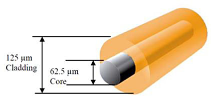
MULTI-MODE FIBER
Multi-mode fiber is the most common fiber type used for network backbone inside buildings. It is the fiber type that the IEEE, ANSI, TIA, and ISO standards typically define in fiber LAN specifications.
The most commonly installed multi-mode core size is 62.5 micrometers (μm). The associated cladding size is 125 μm. But other core sizes are available, like 50 μm, 100 μm, 62.5/125 μm, and 50/125 μm.
Multi-mode features:
- Multiple light paths
- Relatively inexpensive
- Modal-bandwidth limited
- Primarily used for LANs
The ‘multi’ in multi-mode comes from the fact that light travels down the cable in multiple paths. The light beam “bounces” off the cladding as it travels down the core. That means that signals do not necessarily arrive at the receiver at the same instant. Called “modal dispersion”, it is the reason multi-mode fiber has less range than single-mode.
There are two distinct multi-mode methods:
- Step index –
light path is irregular and highly angular - Graded index –
light path is sinuous and regular
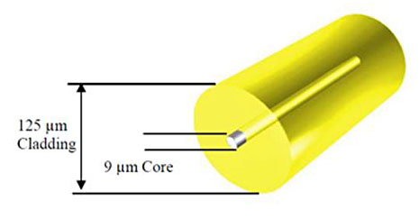
SINGLE-MODE FIBER
Single-mode fiber is used in more demanding applications. Single-mode uses a smaller core diameter (between 8 and 12 μm, with 9 μm being the average) and the same cladding diameter as multi-mode fiber.
Single-mode features:
- 9/125 μm
- Single light path
- Somewhat more costly
- More difficult to terminate
- Essentially unlimited bandwidth
- Primarily used for MAN/WANs
ETHERNET WAVELENGTHS
Fiber optic cables use several different wavelengths to carry Ethernet:
- 850 nm multi-mode – standard for 10Base-FL 10 Mbps Ethernet and 100Base-SX 100 Mbps.
- Short wavelength Ethernet – often used for 1000Base- SX Gigabit Ethernet.
- 1300 nm multi-mode – standard for 100Base-FX 100 Mbps Ethernet. Also used by other high-speed LAN protocols such as FDDI, ATM/OC-3.
- 1310 nm single-mode – standard for 1000Base-LX Gigabit Ethernet. Also commonly used for applications where greater distance is required than can be achieved with multi-mode fiber.
- 1550 nm single-mode – not an Ethernet standard, but used extensively for long-haul telecommunications at speeds of up to 40 Gbps (OC-768).
FIBER STANDARDS
The following table shows the different fiber optic standards as defined by the IEEE.
+ 4B5 encoding on Fast Ethernet and Gigabit Ethernet result in actual bit rates of 125 Mbps and 1250 Mbps respectively.
*100Base-SX (short wavelength multi-mode) and 1000Base-LH (long-haul single-mode) are not formally adopted
FIBER TERMINOLOGY
- Launch Power – the amplitude (or energy) of the light as it leaves the fiber transmitter. This energy level is typically measured in decibels relative to 1 mW (dBm).
- Receive Sensitivity – the minimum energy required for the fiber receiver to detect an incoming signal. This energy level is also measured in decibels relative to 1 mW (dBm).
- Receive Saturation – the maximum power that can be input without overdriving the receiver. Overdriving the receiver can create data errors or a failure to detect any data at all. This energy level is measured in decibels relative to 1 mW (dBm).
- Fiber Budget – the result after subtracting the Receive Sensitivity from the Launch Power. Power budgets are not a measure of energy and are measured in decibels (dB).
- Attenuation – Reduction of signal strength during transmission. Attenuation is the opposite of amplification, and is normal when a signal is sent from one point to another. If the signal attenuates too much, it becomes unintelligible, which is why most networks require repeaters at regular intervals. Attenuation is measured in decibels (dB).
- Modal Dispersion (or Intermodal Dispersion) – Occurs in multi-mode fibers because light travels in multiple modes (reflective paths), and each path results in a different travel distance. Modal dispersion is a major distance limitation with multi-mode fiber.
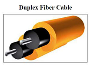
FULL DUPLEX FIBER LOSS AND DISTANCE
To keep it simple, let’s discuss data transmitted over a fiber link is if it were always Full-Duplex (FDX). In a Half-Duplex (HDX) environment, the timing considerations limit the fiber link distances and these limitations apply no matter what fiber is being used.
Since there are two distinct types of fiber cable and three commonly used wavelengths (850 nm, 1300 nm, 1550 nm), the attenuation measurement will vary according to the cable and wavelength being used. Attenuation is measured in dB and is either quoted as attenuation in dB/km, or via an attenuation chart giving the attenuation for the entire fiber run. Note that the decibel scale is logarithmic – a loss of 99% of the light over a given length of fiber is expressed as “-20 dB”, a loss of 99.9% is “-30 dB”, and so forth.
FIBER LOSS VARIABLES
• Attenuation – Fiber cabling has losses from absorption and back reflection of the light caused by impurities in the glass. Attenuation is a function of wavelength and needs to be specified for the particular wavelength in use.
• Modal Dispersion – The higher the data rate, the shorter the distance that the signal can travel before modal dispersion makes it impossible to distinguish between a “1” and “0”. Modal dispersion is only a concern with multi-mode cable and is directly proportional to the data rate.
• Dispersive Losses – While single-mode fiber is not subject to modal dispersion, other dispersion effects cause pulse spreading and limit distance as a function of data rate. Chief among these is “chromatic dispersion,” where the broader spectrum of certain transmitter types can result in varying travel times for different parts of a light pulse. Chromatic dispersion typically only starts to become a limiting factor at Gigabit speeds.
• Splices – Although losses can be small, and often insignificant, there is no perfect lossless splice. Many errors in loss calculations are the result of a failure to include splices. Average splice loss in single-mode cable is usually less than 0.01 dB.
• Connectors – Like splices, there is no perfect lossless connector. It is important to note that even the highest quality connectors can get dirty. Dirt and dust can completely obscure a fiber light wave and create huge losses. Typically, connector loss can vary from 0.15 dB (LC) to 0.5 dB (ST-II). Calculating for a 0.5 dB loss per connector is common and typically represents the worst case scenario, assuming that a cleaned and polished connector is used. Note that there will always be a minimum of two connectors per fiber segment, so remember to multiply connector loss by two.
• Safety Buffer – Add a couple dB of loss as a design margin. Allowing for 2 or 3 dB can account for fiber aging, poor splices, temperature and humidity.
Failure to account for one of these variables can create potential problems. Always test and validate the losses once the fiber is laid. Note that all calculations assume Full-Duplex (FDX) mode of operation.
TYPICAL FIBER LOSS
The numbers listed below are averages and standard for new fiber. Actual numbers may vary for any installation.
CALCULATING SIGNAL LOSS
There are two different calculations required with fiber. Each assumes that there are known values for different sets of variables.
- Maximum signal loss across a piece of pre-existing fiber.
- Maximum fiber distance
given known budget and loss variables.
Calculate maximum signal by loss finding the sum of all worst case variables within a fiber segment. The numbers shown in the table above are average losses. Actual losses could be higher or lower depending upon many factors.
Calculating the signal strength exiting a cable is only half the job. To avoid overdriving a fiber receiver and to eliminate data loss, you must also calculate the “maximum signal strength.” Overdriving a receiver is most common when using single-mode products with very low fiber attenuation. It is safe to assume average numbers for fiber loss but, to verify previous measurements and avoid performance problems, the actual losses should be measured once the fiber has been deployed,
Calculating fiber distance involves the loss variables described above as well as the launch power and receive sensitivity specifications on the fiber products. When calculating distance, use the lowest launch power on the vendor’s specifications to calculate a worst case distance. Use the highest specified launch power to ensure the receiver is not being overdriven.
CALCULATING THE POWER BUDGET
Start by calculating the power budget. This is found by subtracting the receive sensitivity from the launch power.
Power Budget = (Launch Power) - (Receive Sensitivity)
For example, assume a fiber switch with a –17 dBm minimum launch power is connecting to a media converter with a worst case receive sensitivity of 30 dBm:
Power Budget = (-17 dBm) - (-30 dBm) = 13 dB
It may seem odd that subtracting two numbers with dBm as the unit of measure results in a number with dB as the unit of measure. This is because a dBm is a logarithmic ratio of power relative to 1 mW. Subtraction of two logarithmic ratios is the equivalent of dividing the two power measurements directly, resulting in a unitless number expressed in dB.
Because power budgets can be calculated using either decibels or Watts, it is useful to know how to convert between decibels (dBm) and Milliwatts (mW). The two formulas are shown below:
The power budget formula can be expressed in mW rather than dBm. Using the dBm to mW conversion shown above, -17 dBm becomes 0.020mW, -30 dBm becomes 0.001mW and, since subtracting logarithms is the equivalent of dividing two regular numbers, the formula becomes:
Power Budget = 0.020 mW/0.001 mW = 20
This means the system can sustain a total loss of 95% of the transmitted light or that 1/20th of the transmitted light must reach the receiver. The use of dB and dBm as units allows addition and subtraction of reasonably sized numbers rather than multiplication and division of very large or very small numbers.
For a given power budget for 850nm 50 μm multi-mode fiber, and making some assumptions about the number of splices and connections, it is possible to estimate the distance that a fiber with particular specifications can run. For example, using the numbers from above:
If the fiber is specified at a loss not to exceed 2.5 dB/km:
(8.40 dB) / (2.5 dB/km) = 3.36 km
The fiber can be run for approximately 3.36 km (2.1 mi) before running out of signal strength at the end.
A WORD ON MODAL DISPERSION
Multi-mode cable tends to disperse a light wave unevenly and can create a form of jitter as the data traverses the cable. This jitter tends to create data errors as the data rate increases.
In addition to calculating budget across multi-mode fiber, it is also necessary to calculate the losses resulting from modal dispersion. The maximum length of
For example, assume the network is using 100 Mbps Fast Ethernet (which has an actual bit rate of 125 Mbps) across 850 nm multi-mode fiber. The modal dispersion of this multimode cable is 200 MHz-km. Use the following equation to calculate the maximum distance of a 125 Mbps (MHz) Fast Ethernet signal:
Distance = 200 MHz-km/125 MHz = < 1.6 km
Similarly, calculating the maximum distance at a 10 Mbps Ethernet data rate:
Distance = 200 MHz-km/10 MHz = < 20.0 km